Getting started with `JaxILI`#

JaxILI is a python package powered in JAX to perform Neural Density Estimation. It provides a user-friendly interface to run state-of-the-art algorithms of Implicit Likelihood Inference (ILI) also called Simulation-based inference or Likelihood-free inference.

In this tutorial, we show how to get started with JaxILI to perform parameter inference on a simple toy model.

[1]:

import os

import jax
import jax.numpy as jnp
import numpy as np

from jaxili.inference import NPE
from jaxili.model import ConditionalRealNVP

print("Device used by jax:", jax.devices())

2025-04-02 16:00:22.918415: E external/local_xla/xla/stream_executor/cuda/cuda_fft.cc:477] Unable to register cuFFT factory: Attempting to register factory for plugin cuFFT when one has already been registered
WARNING: All log messages before absl::InitializeLog() is called are written to STDERR
E0000 00:00:1743602422.936698  221734 cuda_dnn.cc:8310] Unable to register cuDNN factory: Attempting to register factory for plugin cuDNN when one has already been registered
E0000 00:00:1743602422.942074  221734 cuda_blas.cc:1418] Unable to register cuBLAS factory: Attempting to register factory for plugin cuBLAS when one has already been registered

Device used by jax: [CudaDevice(id=0)]

Implicit Likelihood Inference in a nutshell#

Any Implicit Likelihood Inference algorithm requires three things:

An observational data $x_{\rm obs}$ depending on some parameters $\theta$.
A (stochastic) mechanistic model that samples the observation given the parameters: $x_{\rm obs} \sim p(x|\theta)$. We will refer to it as the simulator.
A prior knowledge of the parameters: $p(\theta)$.

According to Bayes theorem:

\[p(\theta|x)\propto p(x|\theta)p(\theta)\]

Thus, estimating the value of the parameters conditioned on some observational data $x_{\rm obs}$ targets the posterior distribution $p(\theta|x_{\rm obs})$. This can be done using Neural Posterior Estimation trained on the simulator output. If you are new to Implicit Likelihood Inference, please check the `user guide <>`__ (TBD) to familiarize yourself with the theory behind Implicit Likelihood Inference.

The linear Gaussian example#

This illustrative example considers a simulator that takes 3 parameters $\theta$ in input. The likelihood modeled by the simulator follows a simple Gaussian distribution:

\[x|\theta \sim \mathcal{N}(m_{\theta} = \theta, S=0.1 \odot I)\]

This standard problem is part of the SBI benchmark done in Lueckmann et al.. For the sake of simplicity, we will here reduce the dimensionality from $n=10$ to $n=3$. We will consider a uniform prior between -2 and 2: $:nbsphinx-math:`mathcal{U}`(-2, 2).

Let’s first define the simulator:

[2]:

n_dim = 3

def simulator(theta, rng_key):
    batch_size = theta.shape[0]
    return theta + jax.random.normal(rng_key, shape=(batch_size, n_dim))*0.1

Creating the dataset#

We can first draw parameters from the prior to create a dataset of pairs $(\theta_n, x_n)_n$.

[3]:

master_key = jax.random.PRNGKey(0)
num_samples = 10_000

theta_key, master_key = jax.random.split(master_key)

#Draw the parameters from the prior
theta = jax.random.uniform(theta_key, shape=(num_samples, n_dim), minval=jnp.array([-2., -2., -2.]), maxval=jnp.array([2., 2., 2.]))

sim_key, master_key = jax.random.split(master_key)
x = simulator(theta, sim_key)

[4]:

print("Parameters shape:", theta.shape)
print("Data shape:", x.shape)

Parameters shape: (10000, 3)
Data shape: (10000, 3)

Creating the trainer and loading the simulations#

We then need to instantiate an inference object. In this example, we will use Neural Posterior Estimation (NPE).

[5]:

inference = NPE()

We then need to push the simulations in the inference object.

[6]:

inference = inference.append_simulations(theta, x)

[!] Inputs are valid.
[!] Appending 10000 simulations to the dataset.
[!] Dataset split into training, validation and test sets.
[!] Training set: 7000 simulations.
[!] Validation set: 2000 simulations.
[!] Test set: 1000 simulations.

Training#

We can then start to train a Normalizing flow to learn the posterior. A default setup for the training hyperparameters and the model is already in place but it will be shown in other examples (TBD) how to do it.

[7]:

#Specify a checkpoint to save the weights of the neural network
CHECKPOINT_PATH = "."
#Turn it into an absolut path
CHECKPOINT_PATH = os.path.abspath(CHECKPOINT_PATH)

num_epochs = 500

metrics, density_estimator = inference.train(
    checkpoint_path=CHECKPOINT_PATH,
    num_epochs=num_epochs,
)

[!] Creating DataLoaders with batch_size 50.
[!] Building the neural network.

/home/sacha/anaconda3/envs/test/lib/python3.12/site-packages/jaxili/inference/npe.py:352: UserWarning: An embedding net has been specified but not its hyperparameters. Creating an embedding of the instance `Identity` instead.
  warnings.warn("An embedding net has been specified but not its hyperparameters. Creating an embedding of the instance `Identity` instead.")

[!] Creating the Trainer module.
Could not tabulate model:
[!] Training the density estimator.

Epochs: Val loss -2.695/ Best val loss -2.732:   8%|▊         | 38/500 [00:15<03:09,  2.44it/s]
WARNING:absl:`StandardCheckpointHandler` expects a target tree to be provided for restore. Not doing so is generally UNSAFE unless you know the present topology to be the same one as the checkpoint was saved under.

Neural network training stopped after 39 epochs.
Early stopping with best validation metric: -2.7315189838409424
Best model saved at epoch 18
Early stopping parameters: min_delta=0.001, patience=20
[!] Training loss: -2.6210978031158447
[!] Validation loss: -2.7315189838409424
[!] Test loss: -2.705780267715454

Building the posterior and evaluating#

[ ]:

posterior = inference.build_posterior()

[!] Posterior $p(\theta| x)$ built. The class DirectPosterior is used to sample and evaluate the log probability.

We can then directly sample the parameters using the learned distirbution by the Neural Density Estimator.

[ ]:

#Let's first create an observation
obs_key, master_key = jax.random.split(master_key)
fiducial = jnp.array([[0.5, 0.5, 0.5]])
obs = simulator(fiducial, obs_key)

num_samples = 10_000
sample_key, master_key = jax.random.split(master_key)
samples = posterior.sample(
    x=obs, num_samples=num_samples, key=sample_key
)

Visualisation of the learned posterior#

[ ]:

#We will use getdist to visualise the results
import matplotlib.pyplot as plt
from getdist import plots, MCSamples
%matplotlib inline

[ ]:

labels = [rf'\theta_{i}' for i in range(n_dim)]

samples_gd = MCSamples(samples=samples, names=labels, labels=labels)

g = plots.get_subplot_plotter()

g.settings.figure_legend_frame = False
g.settings.alpha_filled_add = 0.4

g.triangle_plot([samples_gd], filled=True,
                line_args=[
                    {'color': 'blue'}
                ],
                contour_colors=['blue'],
                markers={
                    label: val for label, val in zip(labels, fiducial[0])
                })

plt.show()

Removed no burn in

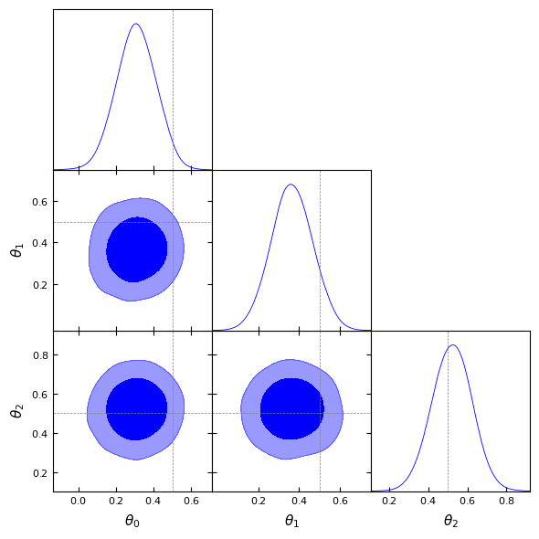
../_images/examples_getting_started_21_1.png

Because of the noise in the simulator and the absence of hyperparameters fine-tuning, it is possible that the ground-truth does not lie at the center of the posterior. This is why it is useful to assess the predictive performance of the psoterior.

[12]:

predictive_key, master_key = jax.random.split(master_key)
x_predictive = simulator(samples, predictive_key)

[13]:

labels = [rf'x_{i}' for i in range(n_dim)]

predictive_samples_gd = MCSamples(samples=x_predictive, names=labels, labels=labels)

g = plots.get_subplot_plotter()

g.settings.figure_legend_frame = False
g.settings.alpha_filled_add = 0.4

g.triangle_plot([predictive_samples_gd], filled=True,
                line_args=[
                    {'color': 'black'}
                ],
                contour_colors=['black'],
                markers={
                    label: val for label, val in zip(labels, obs[0])
                })

plt.show()

Removed no burn in

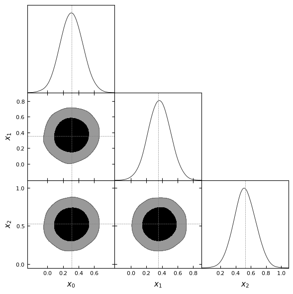
../_images/examples_getting_started_24_1.png

We can see that the posterior predicted is correctly centered on the data. A nice thing about Implicit Likelihood Inference is that the inference is said to be amortiez. It means that the trained network can be used on a different observation without going through the whole training procedure.

[14]:

obs_key, master_key = jax.random.split(master_key)
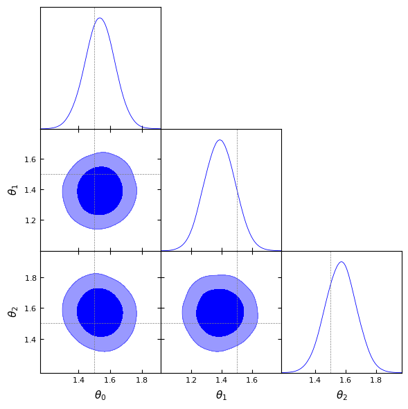
fiducial_2 = jnp.array([[1.5, 1.5, 1.5]])
obs_2 = simulator(fiducial_2, obs_key)

sample_key, master_key = jax.random.split(master_key)
samples_2 = posterior.sample(
    x=obs_2, num_samples=num_samples, key=sample_key
)

[15]:

labels = [rf'\theta_{i}' for i in range(n_dim)]

samples_2_gd = MCSamples(samples=samples_2, names=labels, labels=labels)

g = plots.get_subplot_plotter()

g.settings.figure_legend_frame = False
g.settings.alpha_filled_add = 0.4

g.triangle_plot([samples_2_gd], filled=True,
                line_args=[
                    {'color': 'blue'}
                ],
                contour_colors=['blue'],
                markers={
                    label: val for label, val in zip(labels, fiducial_2[0])
                })

plt.show()

Removed no burn in

../_images/examples_getting_started_27_1.png

[16]:

predictive_key, master_key = jax.random.split(master_key)
x_predictive_2 = simulator(samples_2, predictive_key)

[17]:

labels = [rf'x_{i}' for i in range(n_dim)]

predictive_samples_2_gd = MCSamples(samples=x_predictive_2, names=labels, labels=labels)

g = plots.get_subplot_plotter()

g.settings.figure_legend_frame = False
g.settings.alpha_filled_add = 0.4

g.triangle_plot([predictive_samples_2_gd], filled=True,
                line_args=[
                    {'color': 'black'}
                ],
                contour_colors=['black'],
                markers={
                    label: val for label, val in zip(labels, obs_2[0])
                })

plt.show()

Removed no burn in

../_images/examples_getting_started_29_1.png

Using a non-default architecture#

When creating the inference object, it is possible to choose the architecture of the Normalizing Flow you want to use as well as its hyperparameters.

[18]:

model_class = ConditionalRealNVP
model_hparams = {
    "n_in": n_dim,
    "n_cond": n_dim,
    "n_layers": 3,
    "layers": [50, 50],
    "activation": jax.nn.relu
}

inference = NPE(model_class=model_class, model_hparams=model_hparams)

inference = inference.append_simulations(theta, x)

#Specify a checkpoint to save the weights of the neural network
CHECKPOINT_PATH = "."
#Turn it into an absolut path
CHECKPOINT_PATH = os.path.abspath(CHECKPOINT_PATH)

num_epochs = 500

metrics, density_estimator = inference.train(
    checkpoint_path=CHECKPOINT_PATH,
    num_epochs=num_epochs,
)

[!] Inputs are valid.
[!] Appending 10000 simulations to the dataset.
[!] Dataset split into training, validation and test sets.
[!] Training set: 7000 simulations.
[!] Validation set: 2000 simulations.
[!] Test set: 1000 simulations.
[!] Creating DataLoaders with batch_size 50.
[!] Building the neural network.
[!] Creating the Trainer module.
Could not tabulate model: float() argument must be a string or a real number, not '_ArrayRepresentation'

WARNING:absl:Configured `CheckpointManager` using deprecated legacy API. Please follow the instructions at https://orbax.readthedocs.io/en/latest/api_refactor.html to migrate.

[!] Training the density estimator.

Epochs: Val loss -2.618/ Best val loss -2.634:  28%|██▊       | 139/500 [02:32<06:34,  1.09s/it]

Neural network training stopped after 140 epochs.
Early stopping with best validation metric: -2.6341469287872314
Best model saved at epoch 119
Early stopping parameters: min_delta=0.001, patience=20
[!] Training loss: -2.68935227394104
[!] Validation loss: -2.6341469287872314
[!] Test loss: -2.7200582027435303

[19]:

posterior = inference.build_posterior()

[!] Posterior $p(\theta| x)$ built. The class DirectPosterior is used to sample and evaluate the log probability.

[20]:

num_samples = 10_000
sample_key, master_key = jax.random.split(master_key)
samples = posterior.sample(
    x=obs, num_samples=num_samples, key=sample_key
)

[21]:

labels = [rf'\theta_{i}' for i in range(n_dim)]

samples_gd = MCSamples(samples=samples, names=labels, labels=labels)

g = plots.get_subplot_plotter()

g.settings.figure_legend_frame = False
g.settings.alpha_filled_add = 0.4

g.triangle_plot([samples_gd], filled=True,
                line_args=[
                    {'color': 'blue'}
                ],
                contour_colors=['blue'],
                markers={
                    label: val for label, val in zip(labels, fiducial[0])
                })

plt.show()

Removed no burn in

../_images/examples_getting_started_35_1.png

[22]:

predictive_key, master_key = jax.random.split(master_key)
x_predictive = simulator(samples, predictive_key)

[23]:

labels = [rf'x_{i}' for i in range(n_dim)]

predictive_samples_gd = MCSamples(samples=x_predictive, names=labels, labels=labels)

g = plots.get_subplot_plotter()

g.settings.figure_legend_frame = False
g.settings.alpha_filled_add = 0.4

g.triangle_plot([predictive_samples_gd], filled=True,
                line_args=[
                    {'color': 'black'}
                ],
                contour_colors=['black'],
                markers={
                    label: val for label, val in zip(labels, obs[0])
                })

plt.show()

Removed no burn in

../_images/examples_getting_started_37_1.png

Next steps#

TBD.

Getting started with JaxILI

Contents

Getting started with `JaxILI`#

Implicit Likelihood Inference in a nutshell#

The linear Gaussian example#

Creating the dataset#

Creating the trainer and loading the simulations#

Training#

Building the posterior and evaluating#

Visualisation of the learned posterior#

Using a non-default architecture#

Next steps#

Getting started with JaxILI

Contents

Getting started with JaxILI#

Implicit Likelihood Inference in a nutshell#

The linear Gaussian example#

Creating the dataset#

Creating the trainer and loading the simulations#

Training#

Building the posterior and evaluating#

Visualisation of the learned posterior#

Using a non-default architecture#

Next steps#

Getting started with `JaxILI`#